What makes game engine development complicated is the various algorithms that you need to implement. There is an algorithm used for numerical integration. There is another one to detect collision among convex objects. There is another to compute the collision contact manifold, etc. What is more impressive is that some of these algorithms are simple to understand but complicated to implement.
Most game engine development books explain the Runge-Kutta Method from the mathematical point of view without providing any visual depiction. In this post, I will not focus on the mathematical point of view but the visual point of view. Hopefully, it will give you a better sense of how each algorithm works.
4th Order Runge-Kutta Method
One goal of a physics engine is to compute acceleration, velocity, and displacement from a given Force. It does this by numerically integrating the equation of motion. The simplest numerical integration method that calculates the equation of motion is the Euler's Method.
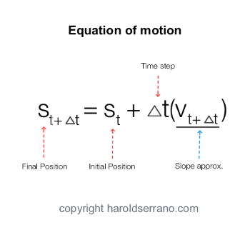
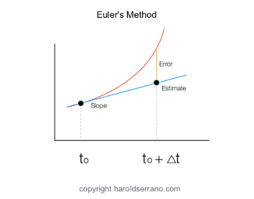
The Euler's Method calculates the velocity at a time interval and predicts the next velocity at t+∆t. The method is simple to implement yet it is the least accurate.The illustration below shows the shortcoming of this approach. You can argue that making ∆t smaller, the closer you'll get to the exact solution. However, there is a practical limit as to how small a time step you can take.
The Runge-Kutta Method is a numerical integration technique which provides a better approximation to the equation of motion. Unlike the Euler's Method, which calculates one slope at an interval, the Runge-Kutta calculates four different slopes and uses them as weighted averages.
These slopes are commonly referred as k1, k2, k3 and k4, and your physics engine needs to compute them at every time step.
Visually, these slopes are calculated as follow:
1) At time interval t0, calculate slope k1.
2) Create a triangle by projecting k1 to t+∆t.

3) Calculate half the height of the triangle, (∆t/2) k1, and draw a horizontal line.
4) Draw a vertical line at interval t+(1/2)∆t.
5) At this intersection point, calculate the slope k2.

6) Starting out with k2, create a triangle by projecting k2 to t+(3/2)∆t.
7) Calculate half the height of the triangle, (∆t/2)k2.

8) Translate the height to the base of the triangle formed by k1 at t+(1/2)∆t.
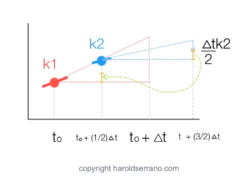
9) At this point, calculate the slope k3.

10) Create the another triangle by projecting k3 to t+(3/2)∆t
11) Find half the height of the triangle, (∆t/2)k3

12) Translate this height to the base of the triangle formed by k1 at point t+∆t

13) Find the slope k4.

The Runga-Kutta uses these slopes as weighted average to better approximate the actual slope, velocity, of the object. The position of the object is then calculated using this new slope.

I hope this visual depiction of the Runge-Kutta method helps.
